• $n(t)$ … (measured, known) number accidents per year $t\in{\mathbb N}$

• $n^\mathrm{max}(t)$ … (unknown) number accidents that would happen without a particular driver assistant systems. As the system prevent some accidents, we have $n(t) < n^\mathrm{max}(t)$.

• $n_\mathrm{prev}(t) = n^\mathrm{max}(t) - n(t)$ … (unknown) number of accidents of $n^\mathrm{max}(t)$, that were prevented, resulting in $n(t)$

• $n_\mathrm{prev}^\mathrm{max}(t)$ … (unknown) number of accidents of $n^\mathrm{max}(t)$, that would be prevented if every car had implemented said system.

• $p := \dfrac{ n_\mathrm{prev}^\mathrm{max}(t) }{ n^\mathrm{max}(t) }$ … (guess, tested) potential of the system.

• $C(t)$ (known) number of cars on the street

• $C^*(t)$ (partially known) number of cars on the street that have implemented the assistance system. For each system, there was a time $t^*$ when when $C^*(t^*)=0$

• $x(t)=\dfrac{C^*(t)}{C(t)}$ … (partially known) distribution of the driver assistance system.

• $p^\mathrm{eff}(t) := \dfrac{ n_\mathrm{prev}(t) }{ n^\mathrm{max}(t) }$ … (unknown) effective potential of the system.

Let

$M(t)=1-p^\mathrm{eff}$

We have

$M(t)\,n^\mathrm{max}(t) = \left(1-\dfrac{ n_\mathrm{prev}(t) }{ n^\mathrm{max}(t) }\right)n^\mathrm{max}(t) = n^\mathrm{max} - n_\mathrm{prev}(t) = n(t)$

Thus $M(t)$ represents the mitigation factor, taking the worse case number of accidents $n^\mathrm{max}(t)$ to the real number $n(t)$. Furthermore, let

$W(t) := \dfrac{1}{M(t)} = \dfrac{1}{1-p^\mathrm{eff}}$

denote the worsening factor, so that

$W(t)\, n(t) = n^\mathrm{max}(t)$

As $n(t)$ can be empirically available, evaluation of $W(t)$ will be more relevant than of $M(t)$.

The distribution $x(t)\le 1$ affects the effective potential. W.r.o.g., we may let

$p^\mathrm{eff} = \Sigma(t)\,x(t)\,p$

where $\Sigma(t)\in(0,1)$ captures all other effects that negatively effect the effective potential. In the following, we'll assume the reduced distribution is the only reason for a reduced potential, i.edeviation(t)=1$. Thus

$W(t) := \dfrac{1}{1-x(t)\,p}$

Using the geometric series $\frac{1}{1-z}=\sum_{k=0}z^k$, we may look at an approximation

$W(t) \approx 1 + x(t)\,p + \left(x(t)\,p\right)^2 $

We can furthermore consider the expansion of the $W(t)$ in $t$ at $t^*$, where $x(t^*)=0$.

$W(t) \approx 1+x'(t^*)\,p\,(t-t^*)+\left(1+\beta\right)\cdot\left(x'(t^*)\,p\,(t-t^*)\right)^2$

with

$\beta=\dfrac{1}{2}\dfrac{1}{p}\dfrac{x''(t^*)}{x'(t^*)}$

In the following, let the distribution $d$ be known/measured to have the values $x^{**}$ at a time $t^{**}$. Define a linear transformation

$s(t)=\dfrac{t-t^*}{t^{**}-t^*}$,

It's chosen so that $s=0$ correspond to the introduction and $s=1$ to the evaluation of the distribution.

The linear model for $d$ reads

$x(t)=\begin{cases} 0 &\hspace{.5cm} \mathrm{if} \hspace{.5cm} t<t^* \\\\ x^{**}s(t)\hspace{.5cm} &\hspace{.5cm} \mathrm{else} \end{cases}$

However, note that as a distribution with $x(t)\le 1$, for $t>t^{**}$ the approximation must somehow start to become flat. This is improved on below.

As $x''(t)=0$ and thus $\beta=0$ for a second order expansion of $W(t)$ above, we get

$W(t) \approx 1 + p\,x^{**}\,s(t) + (p\,x^{**}\,s(t))^2$

Consider now a whole set of systems indexed by $I=\{\mathrm{FAS}_1, \mathrm{FAS}_2,\dots,\mathrm{FAS}_m\}$

Assuming no two systems correlate, we get

$W(t)=\prod_{i=1}^m\dfrac{1}{1-x_i(t)\,p_i}$

Let's look at a systems that shares the times $t^*$ and $t^{**}$. If we consider the linear approximations for $x_i(t)$, we can get the closed form series expression

$W(t)=\sum_{k=0}^\infty b_k s(t)^k$

where

$b_0=1$

$b_1=\sum_{i=1}^mp_i$

$b_2=\sum_{i\le j}^mp_ip_j$

$b_3=\sum_{i\le j < k}^mp_ip_jp_k$

etc.

Proof scetch by induction:

$\dfrac{1}{1-x}=1+x+x^2+\dots$

$\dfrac{1}{1-x}\dfrac{1}{1-y}=(1+x+x^2+\dots)\cdot(1+y+y^2+\dots)=1+(x+y)+(x^2+xy+y^2)+\dots$

$\dfrac{1}{1-x}\dfrac{1}{1-y}\dfrac{1}{1-z}=(1+(x+y)+(x^2+xy+y^2)+\dots)\cdot(1+z+z^2+\dots)=\dots$

etc.

Warmup: The logistic differential equation

$x'(t) = k \cdot x(t) \, \left( K - x(t) \right)$

is e.g used to model the growth of bacteria density $x(t)$ where there's a maximal capacity $x(\infty)=K$. The proportionality factor $k \cdot x(t)$ says the grows is proportional to what's already there and the second factor $K - x(t)$ makes sure $x(t)$ can't grow beyond $K$. The solutions become flat at infinity, but the initial growth is also starting at minus infinity. For normed distributions, $K=1$.

A more realistic class of models for the distribution of assistance systems, that combines the constant (zero) initial value, then an initial linear growth (unlike the logistic function) and a slow flattening, appears to be

$x(t)=x^*$ for $t\le t^*$.

$x'(t)=A(t)\,(1-x(t-t^*))^{1-q}$ for $t> t^*$

for some real $q$. The function $A(t)$ maybe represents the product attractiveness of the system and $1-x(t-t^*)$ are the fraction of drivers at $t-t^*$ which haven't implemented the system product. The equation makes senses in as far as only those drivers can make the distribution of $d$ grow (and there is no reproduction that would depend on the existing distribution $x(t)$, as in the logistic model).

At the introduction of the system, this model makes for a linear rise for small $t>t^*$ and a flattening $x'(\infty)=0$.

We will assume a constant attractiveness $A$. The differential equation is solved by

$x(t)=1-\left((1-x^*)^q-q\,A\cdot(t-t^*)\right)^\frac{1}{q}$

We'll take a look at the model with $q\mapsto 0$, in which case we have

$x(t)=1-(1-x^*)\,{\mathrm e}^{-A\cdot(t-t^*)}$

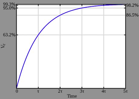
This is the same functional behavior as as resistor voltage step-response in an RL circuit. The linearization for small $t>t^*$ equals

$x(t)\approx x^* + A(t^*)\cdot(t-t^*)$.

If $x(t^{**})=x^{**}$, then

$A=\dfrac{1}{t^{**}-t^*}\log\left(\dfrac{1-x^*}{1-x^{**}}\right)\approx\dfrac{1}{1-x^*}\dfrac{x^{**}-x^*}{t^{**}-t^*}$

and

$x(t)=1-(1-x^*)\left(\dfrac{1-x^{**}}{1-x^*}\right)^{s(t)}$

Indeed, for this function

$x(t^*)=1-(1-x^*)\cdot 1=x^*$

$x(t^{**})=1-(1-x^*)\dfrac{1-x^{**}}{1-x^*}=x^{**}$.

Example for $t^*=2$ and $x^*=0$, $t^{**}=5$ and $x^{**}=0.7$:

https://www.wolframalpha.com/input/?i=1+-+(1+-+0.7)%5E((t+-+2)%2F(5+-+2))+from+0+to+10

We will always have $x^*=0$, as a system can't have any effective potential before it's introduced, so

$x(t) = 1-(1-x^{**})^{s(t)}$

Thus

$W(t) := \dfrac{1}{1-x(t)\,p} = \dfrac{1}{1 - p + (1-x^{**})^{s(t)} p} = L + R$

which splits into the the know linear second order expansion

$L = 1 + p\,x^{**}\,s(t) + (p\,x^{**}\,s(t))^2$

and then some other nonlinear correction terms

$ R \approx (x^{**})^2 \,p\,\left((-p+\frac{1}{2}s)+(p-\frac{1}{2})s^2\right)+\dots$

(At this point the evaluation of the expansion will be more computationally expensiive than using the exact formula with the fraction and exponentials above.)

The presented model predicts that given a maximal potential $p$ for a system introduced at $t^*$ and with a distribution $x^{**}$ at $t^{**}$, the mitigation factor for $t\ge t^*$ giving the relation

$n^\mathrm{max}(t)\,M(t) = n(t)$

is given by

$M(t) = 1 - p + (1-x^{**})^{s(t)} p$

where

$s(t)=\dfrac{t-t^*}{t^{**}-t^*}$

is a linear function. As should be, we have that

$M(t\le t^*) = M(t^*) = 1-\left(1-\left(1-x^{**}\right)^{0}\right)p = 1$

$M(t^{**}) = 1-\left(1-\left(1-x^{**}\right)^1\right)p = 1 - x^{**}\,p$

$M(\infty) = 1-\left(1-0\right)p = 1-p $

Given the above data, the worsening $W(t):=\dfrac{1}{M(t)}$ can be used estimate a would be scenario from empirical accident data $n(t)$.

We considered $p^\mathrm{eff}(t)=x(t)\,\Sigma(t)\,p$. Unknown effects $\Sigma(t)$ may be included in form of a stochastic deviation around the car distribution. We'll introduce a term $\propto\sigma\,{\mathcal W}_t$ to the time evolution of $p^\mathrm{eff}(t)$, where $\sigma$ is a positive real parameter, ${\mathcal W}_t$ a Wiener process and we must do it in such a way that $x(t)\,\Sigma(t)\in[0,1]$.

To this end we take the differential equation

$x'(t) = A\,(1-x(t))$

i.e.

${\mathrm d}x(t) = A\,(1-x(t))\,{\mathrm d}t$

with

$A=-\dfrac{1}{t^{**}-t^*}\log(1-x^{**})$

to

${\mathrm d}X_t = A\,\left[(1-X_t)\,{\mathrm d}t+\sigma\,(4\,X_t\,(1-X_t))^r\,{\mathrm d}{\mathcal W}_t\right]$

with e.g. $r=\frac{1}{2}$.

A expression $4\,X_t\,(1-X_t)\in[0,1]$ is a variation of the stochastic term of the Cox–Ingersoll–Ross-like differential equation (I added a quadratic factor in the distribution with the stochastic term so that it never exceeds $d=1$).

This turns the worsening

$W_t=\dfrac{1}{1-X_t\,p}$

into a stochastic processes. (Or rather a family of such processes, parametrized by $\sigma$ and the standard deviation of the Wiener process.)

For related information, see the simpler Ornstein–Uhlenbeck process with the solution

$X_{t-t^*} = 1-\exp(-A\,(t-t^*)) + \sigma\, {\mathrm e}^{-A\,(t-t^*)}\int_{t^*}^t{\mathrm e}^{+A\,(s-t^*)}\,{\mathrm d}{\mathcal W}_{t^*-s}$

https://en.wikipedia.org/wiki/Ornstein%E2%80%93Uhlenbeck_process)

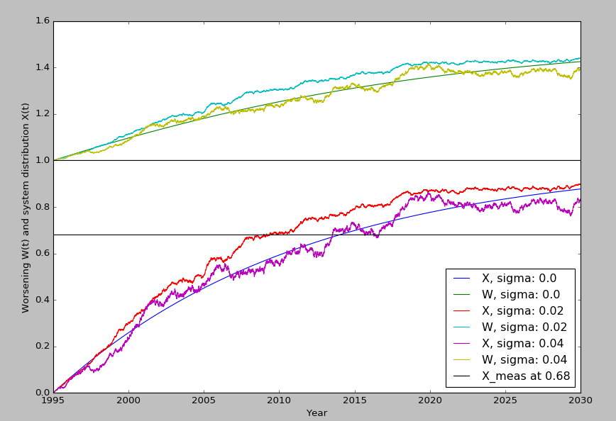
Here we have data for the ESP system, with a distribution of $x^{**}=0.68$ in the year 2014 and thus a slope $A\approx 0.0326$ according to the formula above.

With an estimated (maximal) death reduction potential of $p = 0.34$, the ESP system is the one with the highest $p$ in the list. If all cars had it implemented, $34\%$ of potential deaths would be prevented. In other words, the worsening is $1/(1-0.34)=1.\dot{5}\dot{1}$, meaning if it was never introduced, there would be about $150\%$ as many deaths at this late time. Indeed, removing $34\%$ or those $150\%$ leaves us with the actual $100\%$. Therefore, in the model, we have a stochastic process eventually ending in $X_\infty=1.\dot{5}\dot{1}$. (This is something a linear, without arbitrary cutoff, can't be consistent with.)

The second horizontal line is drawn at $x^{**}$, which intercepts with the $\sigma=0$ curve at $t=2014$. This model still assumes the car distribution eventually reaches 1. The stochastic differential equation, and thus the whole model, can easily be modified to tend towards a maximum $x^\infty<1$ by replacing both expressions $1 - X_t$ with $x^\infty - X_t$.

In the following image, we compute $X_t$ and the associated $W_t$ for $\sigma\in \{0, \frac{1}{100}, \frac{4}{100}\}$ (=$\{0, 0.3, 0.7\}$ after a reparametrization wednesday night). The stochastic variation is implemented via monthly fluctuation, making for $35{\cdot}12$ jumps. The standard deviation of the Wiener process is chosen to be $1$.

import numpy as np
import matplotlib.pyplot as plt
 
p       = 0.34
 
t_intr  = 1995
t_meas  = 2014
X_meas  = 0.68
A       = - np.log(1-X_meas) / (t_meas - t_intr) # equals 0.0326..
 
r              = 1.0 / 2 # small r means smaller penalty on the sides of X=1/2
sigma_Wiener   = 1.0
sigmas         = [0.00, 0.3, 0.7]
 
jumps_per_year = 12
 
t_star = t_intr
t_stop = 2030
N      = (t_stop - t_star) * jumps_per_year
dt     = (t_stop - t_star) / float(N)
t      = np.arange(t_star, t_stop, dt)
 
X      = np.zeros(N)
W      = np.ones(N)
 
for sigma in sigmas:
    for i in xrange(1, t.size):
 
        capac = 1 - X[i-1]
        fluct = sigma * (4 * X[i-1] * capac)**r
        dW    = np.random.normal(loc = 0.0, scale = sigma_Wiener) * np.sqrt(dt)
        X[i]  = X[i-1] + A * (capac * dt + fluct * dW)
 
        W[i] = 1 / (1 - p * X[i])
 
    plt.plot(t, X, label = "X, sigma: " + str(sigma))    
    plt.plot(t, W, label = "W, sigma: " + str(sigma))  
 
plt.plot(t, np.ones(N), color = 'k')
plt.plot(t, np.ones(N) * X_meas, color = 'k', label = "X_meas at " + str(X_meas))
 
plt.ylabel("Worsening W(t) and system distribution X(t)")
plt.xlabel("Year")
plt.legend(loc = 4)
plt.show()

kfv.at

Nikolajs notebook